


Hello,
I’m Élodie, a PhD student on Condenced Matter Theory group on soft matter theory under the direction of Thomas Salez and Yacine Amarouchene .
My researches are to simulate and understand how a Brownian particles is moving near a wall.
I hugely appreciate give some teaching physics and mathematics. Of course, I love vulgarization of science.
I studied fundamental physic, some chemistries specialties and mathematics for PDE and their numerical simulations.
Researches
What is a brownian motion?

Imagine a delicious brownie running through a forest. We know that brownies don’t have a conscience, so he can’t choose his direction of travel and avoid the trees. In the course of its mad dash, it will get its feet caught in the roots and run into the trees, making its trajectory a bit hazardous and perhaps a bit violent for the poor brownie. Finally, if we put a GPS tag on this brownie and record its movement over time, we will observe a random movement. Furthermore, as the forest is uniformly dense, there is no reason why its movement should be favored in a particular direction. In this case, our poor brownie will randomly walk in circles in the forest and never come out! On average, its position will remain its starting point with variations around this position.
In reality, Brownian motion is not that of a brownie! It is rather the movement of a micrometric or nanometric particle, subject to thermal laws that make it random and therefore unpredictable at first sight. In my story, the roots and trees of the forest are the molecules of the fluid in which the particle is immersed and they are agitated by the temperature of the environment. The temperature is the indispensable ingredient at the origin of the random walk of micro particles. However, this effect is no longer effective when the particles are larger. On the right, here is a video showing the preparation and observation of the Brownian motion of micrometric beads.
Observing Brownian motion of micro beads by Forrest Charnock
 « Robert Brown » by Stifts- och landsbiblioteket i Skara is licensed under CC BY 2.0
![]()
![]()
To understand this phenomenon, let’s go back in time. In 1827, Robert was a botanist and explorer. He was one of the first to use the microscope for his work and to classify pollen grains. However, he noticed that once immersed in water, the grains moved randomly without any deterministic movement.
At that time, scientists did not believe Robert (at that time scientists were convinced they had understood everything about the universe), and for a long time rejected his observations, blaming the quality of the microscope’s lenses. Later, it was finally seen that this motion was real and it was called Brownian motion (in honour of Mr Brown for his discovery, not the Brownies of course).
Much later, in 1901, Louis Bachelier worked on a mathematical model of this motion and was the first to lay the first bricks for describing random motion. This research was first applied to finance, which also fluctuates randomly.
Three years later, Albert Einstein highlighted a general law for an erratic particle in free space. He defined the diffusion coefficient which is a constant balance between the fluctuation of the particle due to thermal agitation and its dissipation in space and he indicates in particular that measurements made on the movement make it possible to deduce their molecular size.
Finally, in 1909, Jean Perrin used Albert Einstein’s diffusion model to measure the Avogadro number – the quantity of element in a system containing as many elementary entities as there are atoms in 0.012 kg of carbon 12. Other scientists then went on to develop in more detail the equations of Brownian motion in the case of a free unconstrained particle. This model is now well known.
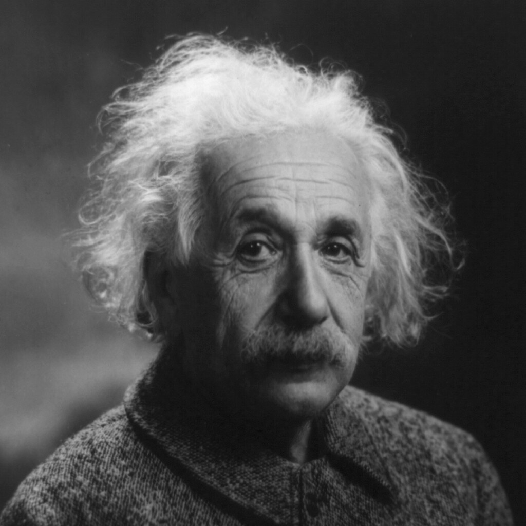 « Albert Einstein » by ThomasThomas (license CC BY-NC 2.0)
![]()
![]()
![]()
What about now?
Currently, we know how to describe the movement of a micrometric particle in bulk space. The big problem with this theory is that nothing is free or far from any other object in nature.
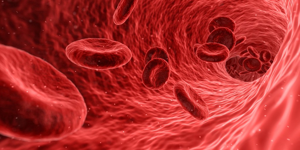 « Red Blood cells » by SciTechTrend (license CC PDM 1.0)
![]()
![]()
Let us take the example of red blood cells in blood vessels. Can we apply these laws in this specific case? We realised that it is not and that many physical phenomena come into play to modulate the equations of Brownian motion. The presence of the blood vessel wall induces a force on the particle, but not only; its own diffusion is impacted by its distance to the vessel wall at each instant. Thus, in this case, the diffusion coefficient of a particle is no longer a constant of the problem, but varies with the distance to the wall.
We also know that there is not just one red blood cell in the blood vessels, so interactions between particles also have an effect. It is around these questions that my research is focused. I am working on the effects of a hard or soft wall and on the interactions between particles.
My researches
Active particle near a soft wall

For a simpler problem, consider a particle close to a rigid wall. It is subject to weight, which attracts it close to the wall, but it is also repelled by the wall due to electron repulsion. The particle is thus confined in the direction transverse to the wall, but free in the collinear directions. In addition, the presence of the wall modifies the friction between the particle and the fluid, resulting in an effective viscosity that increases as the particle approaches the wall, as you can see in the figure below. Since diffusion depends inversely on the viscosity of the fluid, the closer the particle is to the wall, the less it diffuses.

As the particle follows a stochastic trajectory, due to thermal noise, one can study its probability density of presence near the wall.

Figure a) shows the probability of finding the particle at a certain distance from the wall. It is asymmetrical and one can see the most probable position, the confinement distance. On the left, the probability drops drastically as one gets closer to the wall since the electrostatic repulsion of the wall is very strong. On the right, the probability decreases more slowly, because only gravity comes into play.
Figures b) and c) show the probabilities of displacement of the particle, respectively, parallel and perpendicular to the wall when the displacement times τ are short compared to the characteristic time of reaching the thermodynamic equilibrium (where Δx = x(t+τ)-x(t)). In the bulk case (free particle), these probabilities are Gaussian (blue dotted line) and we see that this does not work anymore after adding a rigid wall, even along the axis parallel to the wall.
Figure d) shows this probability at long time and diffusion does not come into play directly anymore.
It can be seen that the theory with the wall is in agreement with my simulations. At short time, large displacements are more probable than in the bulk case because of the wall constraints. At long time, the probability is no longer governed by diffusion.
See more about confined brownian motion near a wall with the PhD manuscript of Maxime Lavaud, who works on experimental approche of this problem.
We know how to discribe trajectory of a brownian particle near a rigid wall. Now the perspectives is to concidere a soft wall, where the dynamic of particle change the wall profil and the wall profil change the movement of the particle.
Taylor-Aris dispersion with hydrodynamic interactions
Incomming soon …
Collaborations
EMetBrown team
 ll
ll
Non-permanent
Zaicheng Zhang, PostDoc
Maxime Lavaud, PostDoc
Aditya Jha, PostDoc
Alexandre Vilquin, PostDoc
Caroline Kopecz Muller, PhD
Élodie Millan, PhD
Nicolas Fares, PhD
Yilin Ye, Master 1 internship
Quentin Ferreira, Master 1 internship
Projects


Curriculum vitae
![]()
Degrees
2020-2023 :
Ph.D. in lasers, matter, nanosciences – Actives particles near a soft wall – LOMA, University of Bordeaux.
2019-2020 :
First year of M.Sc Applied mathematics, statistics, path Partial differential equations and Modeling – University of Bordeaux.
2018-2019 :
M.Sc Fundamental physics and applications, Physics Aggregation course – University of Bordeaux.
2016-2018 :
M.Sc Fundamental physics and applications, Lasers, matter and nanosciences courses – University of Bordeaux..
2015-2016 :
B.Sc Physics – University of Bordeaux.
2013-2015 :
Two years of B.Sc Physics and Chemistry – University of Bordeaux.
Experiences
2020-2022 :
Teaching missions – BSc degree – Optics, Mathematics for Chemistry, Thermodynamics, Electromagnetisme, Vibrations, Calorimetry University of Bordeaux.
2020 :
Reserches intership – Brownian particles near a rigid wall – LOMA, University of Bordeaux.
2018-2019 :
Teaching internship in « Classe préparatoire aux grandes écoles » – Teached in lab class, tutorials and « Khôlles » – Montaigne Hight school, Bordeaux.
2018 :
Reserches intership – Actives particles at interfaces – LOMA, University of Bordeaux.
2017-2019 :
Oral examination jury of second year or B.Sc of physics – University of Bordeaux.
2017 :
Reserches internship – Methanol deutered in a region of Orion nebula – Laboratoire d’Astrophysique de Bordeaux, University of Bordeaux.
2016 :
Reserches internship – Simutation of laser equations – Centre d’étude de laser intence et applications, University of Bordeaux.
Skills
Physics
- Brownian motion,
- Statistical physics,
- Hydrodynamics interactions and Stokesian dynamics,
- Basic in biophysics.
Programming
- :
Python,Cython, basics inC. - : You can visit my Github page.
- Numerical simulations in PDE
Teaching
![]()
2020 – 2021
L1 Science de la Vie et de la Terre – TP d’optique géométrique.
L2 Chimie – TD de méthodes mathématiques pour la chimie.
L2 Physique – TP de thermodynamique.
L3 Cursus Master en Ingénierie IMSAT – TD et TP de vibrations.
2021 – 2022
L2 Chimie – TD de méthodes mathématiques pour la chimie.
L2 Physique – TD et TP d’Électrostatique et Magnétostqtique.
L3 Cursus Master en Ingénierie IMSAT – TD et TP de vibrations.
L1 Cursus Master en Ingénierie IMSAT – TD de Calorimétrie.

Élodie MILLAN
Laboratoire Ondes et Matière d’Aquitaine (LOMA)
351 cours de la libération
33405 Talence Cedex
Phone : + 33 (0)5 40 00 62 09
E-mail: elodie.millan@etu.u-bordeaux.fr
Office : 202